NUMERICAL STUDY OF UNSTEADY CAVITATION CHARACTERISTICS AROUND NACA66 HYDROFOIL USING LES MODEL

V. Karthik; J.C. Lee

doi:10.6112/kscfe.2024.29.1.090

Preview

Original Article

Journal of Computational Fluids Engineering. 31 March 2024. 90-99
https://doi.org/10.6112/kscfe.2024.29.1.090

NUMERICAL STUDY OF UNSTEADY CAVITATION CHARACTERISTICS AROUND NACA66 HYDROFOIL USING LES MODEL

LES 모델을 이용한 NACA66 수중익 주위의 비정상 캐비테이션 특성에 대한 수치해석적 연구

V. Karthik¹

J.C. Lee¹^*

Vadivelu Karthik¹

이 장창¹^*

¹Dept. of Mechanical Engineering, Andong National University

¹안동대학교 기계공학과

^{*Corresponding Author}

ABSTRACT

The presence of cavitation in hydraulic machinery leads to vibrations, noise, and a decrease in efficiency. The characteristics of unsteady partial cavitation around NACA66 hydrofoil are numerically investigated. The Schnerr-Sauer cavitation model which is based on two-phase Rayleigh-plesset equation (bubble transport equation) is applied with LES turbulence model. The stable cavitation characteristics affected by cavitation length are studied. In results, the contours of the the vortical structure, boundary layer separation, the re-entrant jet, and the transition from sheet cavitation to cloud cavitation are clearly shown. The numerical results are in good agreement with the experiment.

Keywords

비정상 캐비테이션(Unsteady Cavitation)

LES 모델(LES model)

NACA66 수중익(NACA66 hydrofoil)

Schnerr-Sauer 캐비테이션 모델(Schnerr-Sauer Cavitation model)

MAIN

1. Introduction
2. Methodology
2.1 Governing Equations
2.2 Numerical Methodology
2.3 Validation
3. Results and Discussion
4. Conclusion

1. Introduction

The cavitation phenomenon usually occurs in hydraulic machineries. As the local pressure of fluid particles goes below the saturation vapor pressure at the given temperature, the liquids are vaporized. The vapor bubbles are collapsed in the high pressure region. This process, the bubble growth and collapse, is highly transient. As each vapor bubble collapses, a strong shock wave is generated and directed towards the nearby surface. These bubble collapses are similar to intense water hammer effect [1]. Over the prolonged period, this results in surface erosion.

Kubota et al. [2] investigate experimentally the unsteady cloud cavitation around a symmetrical hydrofoil. It is shown that a cluster contains many small cavitation bubbles, the vorticity maximum observe at the cluster center, and the convection velocity of the cavitation cloud is much lower than the uniform velocity.

Stutz and Rebound [3] study experimentally the flow structure of sheet cavitation. The sheet cavitation consists of the cavity due to the extended reversed flow along the solid surface. It is a complex two-phase flow. The void fraction of the cavity is also decreased regularly.

Kawanami et al. [4] analyze experimentally the transition process of the sheet cavitation to the cloud cavitation. The collapse of the sheet cavity on the surface of hydrofoil is triggered by a re-entrant jet. As a result, the part of the sheet cavity is shed near the leading edge and flows downstream. This cluster of bubbles is called the cloud cavity.

Leroux et al. [5] conduct experimental analysis for NACA66 hydrofoil with wall-pressure sensors which are installed on the surface of hydrofoil to investigate unsteadiness in partial cavitation. It is found that cavity lengths do not exceed half of the hydrofoil chord where the cavity is stated to be stable. Conversely, the cavities larger than half of hydrofoil chord is stated to be unstable. The unsteadiness around NACA66 hydrofoil surface during a cavity growth/destabilization cycle fluctuates dramatically.

Coutier et al. [6] simulate numerically 2-D unsteady cavitation behavior for a venturi-type duct with source terms calculated for the vaporization and condensation process. This source term is managed by a bartropic state law which relates the fluid density to the pressure variations. On the other hand Merkle et al. [7] study numerically the multiphase cavitation model based on Rayleigh-Plesset equation which is the fundamental equation for spherical bubble dynamics used in the source term to govern evaporation and condensation. Additionally the volume fraction term is introduced to the mass and momentum equation.

Kunz et al. [8], Schnerr & Sauer [9], and Singhal et al. [10] also apply similar techniques with different source terms including the bubble transport equation for their cavitation models.

The turbulence model is essential in numerical studies of cavitation flow because the cavitation is inherently unsteady in nature and the strong interaction between the cavity interface and the boundary layer exists [11]. The Reynolds Average Navier-Stokes(RANS) equation is used to solve the wide range of problems. However, it has limited capabilities and needs modifications for the unsteady cavitation flows at high Reynolds numbers. Large Eddy Simulation(LES) model for cavitation flows are expected to give better predictions of the large turbulent eddies with better accuracy. Ji et al. [11] simulate numerically 3-D unsteady cavitating flow around a twisted hydrofoil with LES turbulence model and shows good agreement with experiment.

In the present numerical study, the characteristics of unsteady partial cavitation around NACA66 hydrofoil are investigated by applying the Schnerr and Sauer cavitation model with LES. The geometry of NACA66 hydrofoil is obtained from the experiment of Leroux et al. [5]. The stable cavitation characteristics influenced by cavitation length are studied. The numerical results are compared with the pressure coefficients of the experiment. The contours of the the vortical structure, boundary layer separation, the re-entrant jet, and the transition from sheet cavitation to cloud cavitation are clearly shown by using the LES turbulence model.

2. Methodology

2.1 Governing Equations

In this paper, the unsteady cavitation flow is solved by Schnerr-Sauer model with LES turbulence model. The fundamental governing equations for the mass and momentum equation are

(1)

\frac{\partial ρ}{\partial t} + \frac{\partial (ρ u_{j})}{\partial x_{j}} = 0

(2)

\frac{\partial (ρ u_{i})}{\partial t} + \frac{\partial (ρ u_{i} u_{j})}{\partial x_{j}} = \frac{\partial p}{\partial x_{i}} + \frac{\partial}{\partial x_{j}} (μ \frac{\partial u_{i}}{\partial x_{j}})

where 𝜌 is the density, $u_{i}$ is the velocity in the $i$ direction, and $p$ is the pressure of the mixture. In the cavitation flow, the fluid density 𝜌 and laminar viscosity 𝜇 are modified by

(3)

ρ = (1 - α_{V}) ρ_{L} + α_{V} ρ_{V}

(4)

μ = (1 - α_{V}) μ_{L} + α_{V} μ_{V}

where $α_{V} (= \forall_{V} / \forall)$ is the vapor volume fraction and the subscripts $L$ and $V$ are liquid and vapor respectively.

Applying a Favre-filtering operation to Eq. (1) and (2) gives the LES equations [11]:

(5)

\frac{\partial ρ}{\partial t} + \frac{\partial (ρ \bar{u_{j}})}{\partial x_{j}} = 0

(6)

\frac{\partial (ρ \bar{u_{i}})}{\partial t} + \frac{\partial (ρ \bar{u_{i}} \bar{u_{j}})}{\partial x_{j}} = - \frac{\partial \bar{p}}{\partial x_{i}} + \frac{\partial}{\partial x_{j}} (μ \frac{\partial \bar{u_{i}}}{\partial x_{j}}) - \frac{\partial τ_{i j}}{\partial x_{j}}

where the over-bars represent the filtered quantities. $τ_{i j}$ is given by

(7)

τ_{i j} = ρ (\bar{u_{i} u_{j}} - \bar{u_{i}} \bar{u_{j}})

which is the Sub-Grid Scale(SGS) stresses. It assumes that the SGS stresses are proportional to the modulus of the strain-rate-tensor, $\bar{S_{i j}}$ , which is the filtered large scale flow. The eddy-viscosity model is the commonly used SGS model. The Eq. (7) is modified as

(8)

τ_{i j} - \frac{1}{3} τ_{k k} δ_{i j} = - 2 μ_{t} \bar{S_{i j}}

where $δ_{i j}$ is the Kronecker symbol and $μ_{t}$ is the SGS turbulent viscosity which is closed by the LES Wall Adapting Local Eddy-Viscosity(WALE) model [12]. The main advantage of WALE model is its ability to reproduce the laminar to turbulent transition and return the correct wall-asymptotic $y^{+ 3}$ -variation of the SGS model.

In the LES, the $q$ -criterion is used to visualize coherent structures, such as vortices, in turbulent flows. It is particularly useful for identifying regions of significant vorticity where turbulence is organized into coherent structures rather than being fully turbulent. The $Q$ -criterion is defined as follows:

(9)

Q = \frac{1}{2} (| ω |^{2} - \frac{{\bar{S_{i j}}}^{2}}{2})

where 𝜔 is the vorticity vector.

Schnerr-Sauer cavitation model is based on Rayleigh-Plesset. The mass transfer equation is given by

(10)

\frac{\partial (ρ_{V} α_{V})}{\partial t} + \frac{\partial (ρ_{V} α_{V} u_{j})}{\partial x_{j}} = {\dot{m}}^{+} - {\dot{m}}^{-}

where the source terms ${\dot{m}}^{+}$ and ${\dot{m}}^{-}$ represents the effects of vaporization and condensation process. The source terms in Eq. (9) are defined as follows :

when $p < p_{V}$ ,

(11)

{\dot{m}}^{+} = \frac{ρ_{V} ρ_{L}}{ρ} α_{V} (1 - α_{V}) \frac{3}{R_{b}} \sqrt{\frac{2 (p_{V} - p)}{3 ρ_{L}}}

and when $p > p_{V}$ ,

(12)

{\dot{m}}^{-} = \frac{ρ_{V} ρ_{L}}{ρ} α_{V} (1 - α_{V}) \frac{3}{R_{b}} \sqrt{\frac{2 (p - p_{V})}{3 ρ_{L}}}

where the subscripts $V$ and $L$ are vapor and liquid respectively. The $α_{V}$ is the vapor volume fraction. $N_{b}$ is the bubble number density. $R_{b}$ is the radius of the bubble which is

(13)

R_{b} = (\frac{α_{V}}{1 - α_{V}} \frac{3}{4 Π} \frac{1}{N_{b}})^{1 / 3} .

The $N_{b}$ is specified as 10¹³ according to the Schnerr-Sauer model [9].

2.2 Numerical Methodology

A finite volume approach using ANSYS Fluent 23. R2 solves the 3-D unsteady cavitation flow. The multiphase mixture model is solved by the implicit method. The energy equation is not solved because the cavitation process is considered to be iso-thermal for water. In the viscous model, the LES coupled with the WALE SGS model is adapted in this paper. For the spatial discretization, the Least Squares Cell Based is used to calculate the gradient, the Bounded Central Differencing scheme is used in the momentum, and the QUICK method is used in the volume fraction. The Bounded Second Order Implicit method is used in the transient formulation.

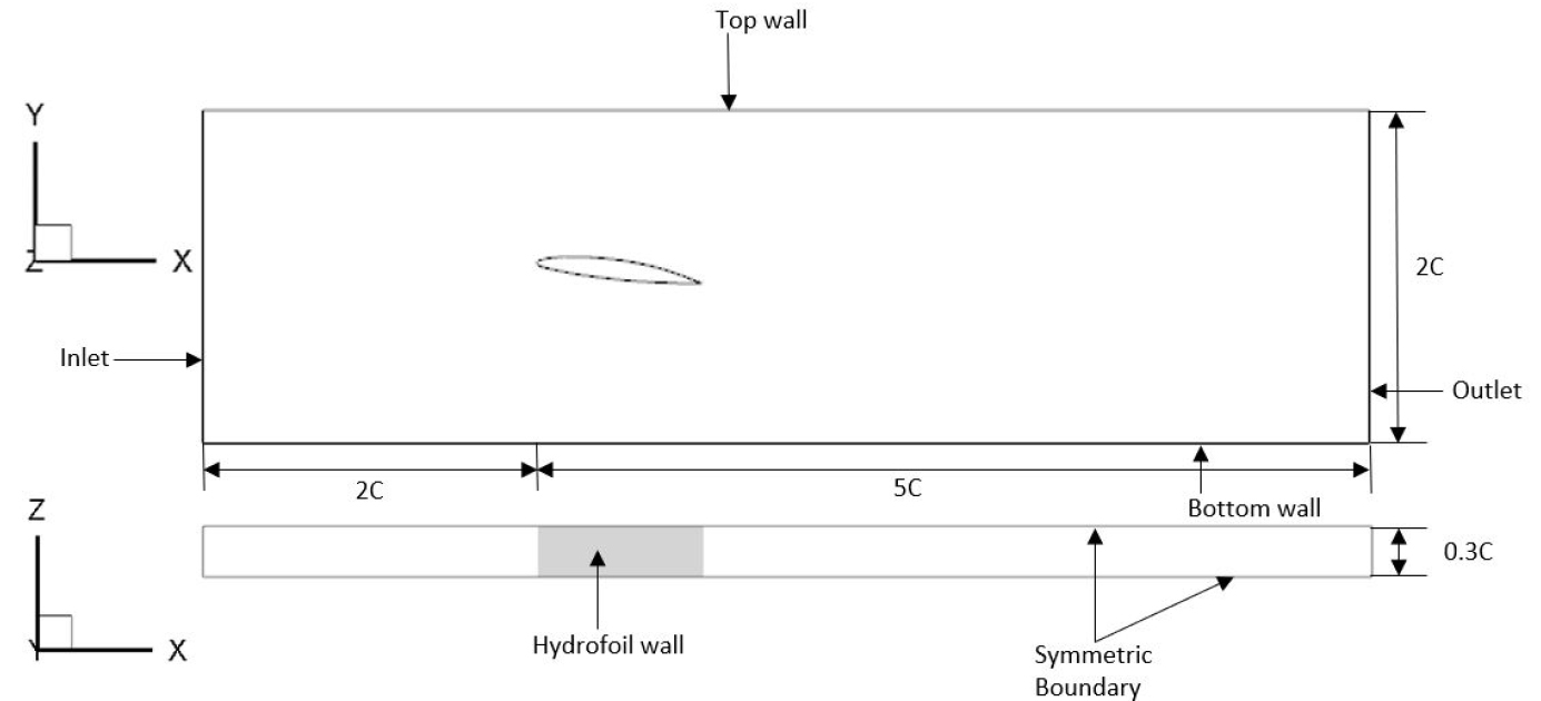
The computation domain around the cambered NACA66 hydrofoil which has the relative maximum thickness of 12% and a relative maximum camber of 2% is shown in Fig. 1 where the chord length of hydrofoil is C = 0.15 m and the angle of attack (𝛼) is 6 degrees. The span-wise length is chosen as 0.3C, which is more than twice the foil thickness sufficient to resolve the stream-wise vortices [13]. The inlet and outlet is located at the distance of 2C and 5C respectively from the leading edge. The height is sufficiently set to 2C to avoid wall effect.

https://cdn.apub.kr/journalsite/sites/kscfe/2024-029-01/N0500290108/images/jkscfe_29_01_08_F1.jpg

Fig. 1.

Computational domain with the boundary conditions

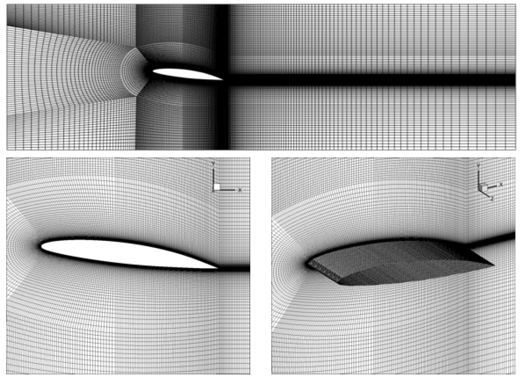
The LES must resolve a large portion of high wave-number turbulent fluctuations. This requires either high-grid resolution if low order schemes are used or high-order numerical schemes is required. In this paper, a high resolution O-H type mesh is used for the computation domain shown in Fig. 2 with sufficient refinement near the hydrofoil surface. The wall $Y^{+}$ value should be less than 1 for the LES. Here, it is $Y^{+}$ $\approx$ 0.7 and the distance from the wall for the first grid is 3.0×10^-6 [m]. The total number of grids is 3.4 million cells and the number of cells in streamwise and spanwise on the surface of hydrofoil is 300×60 cells.

https://cdn.apub.kr/journalsite/sites/kscfe/2024-029-01/N0500290108/images/jkscfe_29_01_08_F2.jpg

Fig. 2.

Mesh generation around NACA66 hydrofoil

The uniform free-stream inlet velocity is $V_{\infty} =$ 5.33 m/s with no perturbations. The outlet pressure is adjusted to vary the cavitation number given by the formula ( $σ = (p_{\infty} - p_{V}) / 0.5 ρ_{L} V_{\infty}^{2}$ ) where $p_{V}$ is the saturated vapor pressure and is set as 2350 [Pa] for the given temperature $T$ =293.15 [K], $ρ_{L}$ is the density of the water, and $p_{\infty}$ is the pressure at the outlet.

The simulations for unsteady cavitating flow are initially started with the converged solution for the unsteady non-cavitating flow. The time step size is set 1.0×10^-4 [s]. The calculations are performed in a computer with Intel Core i9-13900K CPU which contains 24 cores and with 128GB of RAM.

2.3 Validation

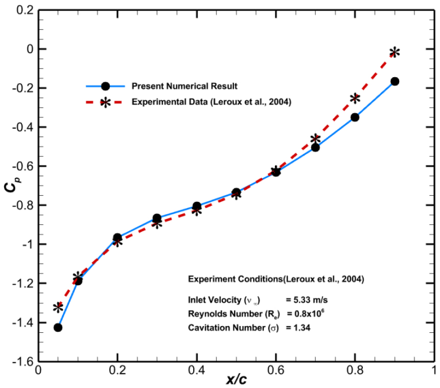
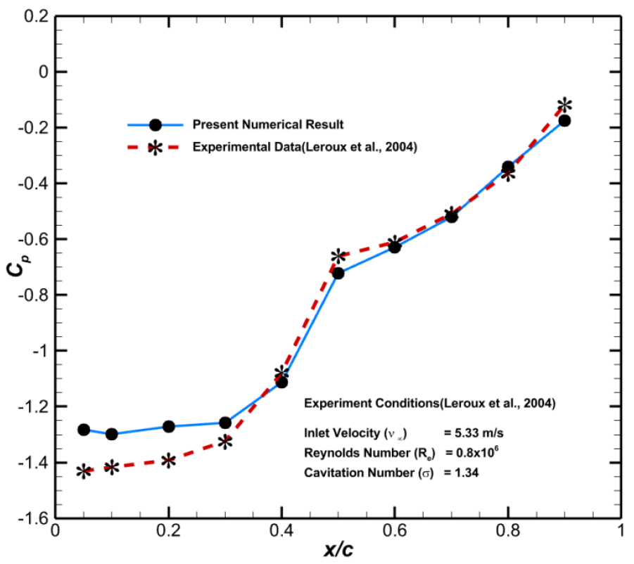
The present numerical model is validated with the experimental case for NACA66 hydrofoil [5] where the free-stream inlet velocity is $V_{\infty}$ =5.33 [m/s], Reynolds number is $R_{e} = 0.8 \times 10^{6}$ , the cavitation number is 𝜎=1.34, and the angle of attack (𝛼) is 6 degrees. The comparison of pressure coefficient with the experimental values of NACA66 hydrofoil is shown in Fig. 3 for unsteady non-cavitating flow and in Fig. 4 for unsteady cavitating flow. The pressure points are the same as the pressure transducer locations mounted on the suction side of hydrofoil surface [5]. In the present numerical results, the $C_{p}$ is calculated with the time-averaged mean value because the transient pressure for unsteady flow are oscillated. The point, $x / c = 0.5$ , is the inflection point in Fig. 3. On the left-hand side of $x / c = 0.5$ , the $∆ p$ increases gradually but on the right-hand side, the slope of $∆ p$ is more stiff. In Fig. 4, the $C_{p}$ also shows a different trend after $x / c = 0.5$ . This phenomenon is caused by periodic growth and collapse of vapor regions on the suction side of the hydrofoil (see Fig. 5). When the experimental values of $C_{p}$ at $x / c = 0.2$ are compared, $C_{p}$ (=-1.392) for the cavitating flow is 44.7% lower than $C_{p}$ (=-0.96217) for the non-cavitating flow because of the cavitation as a vapor-block which makes the flow slow. The numerical results of $C_{p}$ at $x / c = 0.7$ for both non-cavitating flow ( $C_{p}$ =-0.516) and cavitating flow ( $C_{p}$ =-0.519) are similar. It can be observed that the current Schnerr-Sauer cavitation model is consistent with the experimental data.

https://cdn.apub.kr/journalsite/sites/kscfe/2024-029-01/N0500290108/images/jkscfe_29_01_08_F3.jpg

Fig. 3.

Comparison of C_p with experimental data for unsteady non-cavitating flow

https://cdn.apub.kr/journalsite/sites/kscfe/2024-029-01/N0500290108/images/jkscfe_29_01_08_F4.jpg

Fig. 4.

Comparison of C_p with experimental data for unsteady cavitating flow

https://cdn.apub.kr/journalsite/sites/kscfe/2024-029-01/N0500290108/images/jkscfe_29_01_08_F5.jpg

Fig. 5.

Snapshots of the cavitation shedding in 3D and 2D

3. Results and Discussion

The characteristics of the attached cavity length around NACA66 hydrofoil is determined by the cavitation number(𝜎) [5]. If $σ ≺$ 1.3, the flow makes the unstable cavitation where the attached cavity length is more than half of the chord length. Conversely, if $σ ≻$ 1.3, it is called the stable cavitation where the attached cavity length is less than half of the chord length.

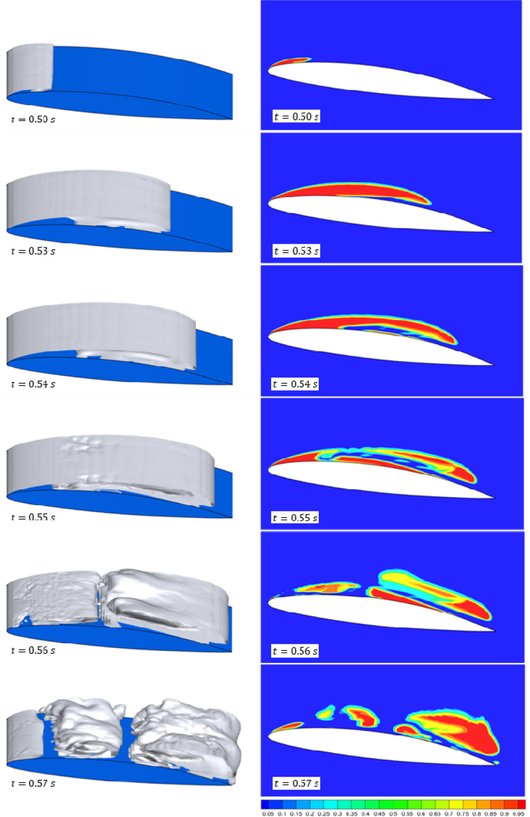
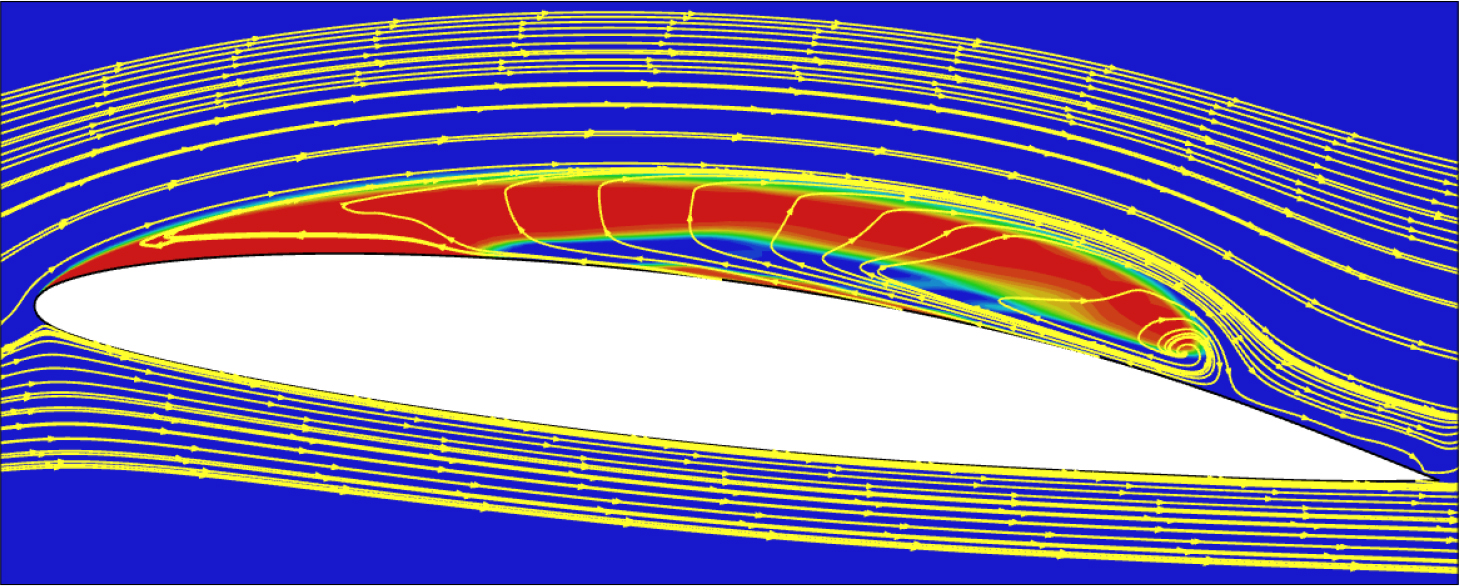
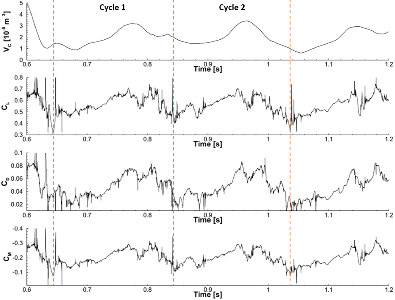
The unsteady caviting flow around NACA66 hydrofoil is investigated with 𝜎=1.34 in this paper. Fig. 5 shows the cavity shape evolution and the contours of vapor volume fraction in one typical cavitation cycle. It is seen that a short cavity sheet is developed from the leading edge at the instant of $t$ =0.50 [s]. The attached sheet cavity grows to $x / c = 0.4$ and the sheet cavity is detached by the re-entrant jet at the instant of $t$ =0.53 [s] (see Fig. 6). The re-entrant jet arrives at $x / c = 0.3$ and collides with the cavity sheet at the instant of $t$ =0.55 [s]. A cloud cavity starts to generate and the shedding cloud cavity is further convected downstream at the instant of $t$ =0.57 [s]. Fig. 6 represents the streamlines around NACA66 hydrofoil where the re-entrant jet formation and the vortex flow can be verified. The total length of spanwise is 0.045 [m]. The origin point is located in the middle of the span. Fig. 7 shows the periodic variations of cavity volume (V_C), lift, drag, and moment coefficient in the meantime of unsteady calculations. Here, the total volume of vapor volume fraction is defined as the cavity volume. Two periodic cycles are found in all graphs. The curves for the lift, drag, and moment coefficient are oscillated due to the combination effects of cavitation activity and turbulence fluctuations, which is not perceivable from the cavity volume curve.

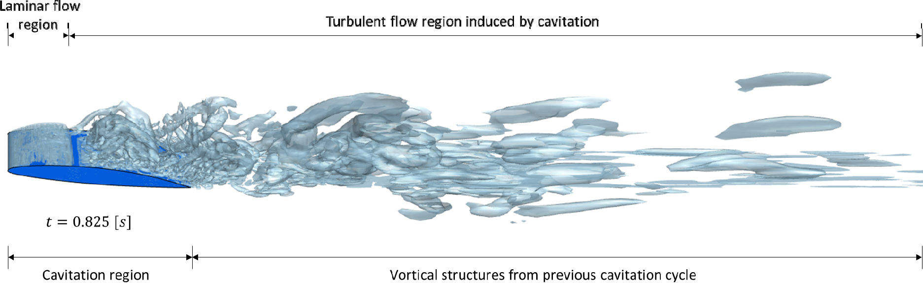
Fig. 8 shows the coherent vortical flow structure in the wake region. The previous shedding cloud cavitation creates vorticity and turbulent flow in the wake region. The $Q$ -criterion is used to identify and quantify regions of significant vorticity or rotation within a fluid flow field. The vorticity represents the local spinning or swirling motion of fluid particles. It plays a crucial role in the dynamics of turbulent flows, especially in the LES model. The $Q$ - criterion is defined $Q = 10^{3} [s^{- 2}]$ . Two transition phenomena are observed in this figure. One is the transition between the laminar and turbulent flow and the other one is the transition between the sheet and cloud cavitation on the surface of NACA66 hydrofoil caused by re-entrant jet. The previously shedded cloud cavitation cycle has a great effect in the wake region where the vortical structures cause the periodic shedding of cloud cavitation.

https://cdn.apub.kr/journalsite/sites/kscfe/2024-029-01/N0500290108/images/jkscfe_29_01_08_F6.jpg

Fig. 6.

Streamlines at the instant of t=0.54 [s] in spanwise ( +0.0225 [m])

https://cdn.apub.kr/journalsite/sites/kscfe/2024-029-01/N0500290108/images/jkscfe_29_01_08_F7.jpg

Fig. 7.

Periodic variations of cavity volume and force coefficient in the meantime of unsteady calculations

https://cdn.apub.kr/journalsite/sites/kscfe/2024-029-01/N0500290108/images/jkscfe_29_01_08_F8.jpg

Fig. 8.

Vortical structures and wake vortices induced by cavity shedding (iso-surfaces of $Q = 10^{3} [s^{- 2}]$ , $σ = 1.34$ , $α = 6 °$ )

4. Conclusion

The numerical simulation is performed to study the effect of stable cavity formation and collapsing around NACA66 hydrofoil. The following conclusions are given:

1. The Schnerr-Sauer cavitation model for unsteady cavitating flow around NACA66 hydrofoil with 𝜎=1.34 is consistent with the experimental data.

2. The behavior of cavity shape evolution around the foil for the stable cavitation is well predicted.

3. The curves for the force coefficient are oscillated due to the combination effects of cavitation activity and turbulence fluctuations, which is not perceivable from the cavity volume curve.

4. The $Q$ -criterion is used to visualize coherent structures in turbulent flows by using the LES model.

Acknowledgements

This work was supported by a Research Grant of Andong National University.

References

2009, Wright, T. and Gerhart, P.M., "Fluid Machinery-Application, Selection, and Design," CRC Press.

1989, Kubota, A., Kato, H., Yamaguchi, H. and Maeda, M., "Unsteady Structure Measurement of Cloud Cavitation on a Foil Section using Conditional Sampling Technique," J. Fluids Eng., Vol.111, pp.204-210. 10.1115/1.3243624

1997, Stutz, B. and Reboud, J.L., "Two-phase Flow Structures of Sheet Cavitation," Phys. Fluids, Vol.9, pp.3678-3686. 10.1063/1.869505

1997, Kawanami, Y., Kato, H., Yamaguchi, H., Tanimura, M. and Tagaya, Y., "Mechanism and Control of Cloud Cavitation," J. Fluids Eng., Vol.119, pp.788-794. 10.1115/1.2819499

2004, Leroux, J.B., Astolfi, J.A. and Billard, J.Y., "An Experimental Study of Unsteady Partial Cavitation," J. Fluids Eng., Vol.126, pp.94-101. 10.1115/1.1627835

2003, Coutier, D.O., Reboud, J.L. and Delannoy, Y., "Numerical Simulation of the Unsteady Behaviour of Cavitating Flows," Int J. Numerical Methods in Fluids, Vol.42, pp.527-548. 10.1002/fld.530

1998, Merkle, C.L., Feng, J.Z. and Buelow, P.E., "Computational Modeling of the Dynamics of Sheet Cavitation. In: Proceedings of the Third International Symposium on Cavitation," Grenoble, France.

2000, Kunz, R.F., Boger, D.A., Stinebring, D.R., Chyczewski, T.S., Lindau, J.W., Gibeling, H.J.,Venkateswaran, S. and Govindan, T.R., "A Preconditioned Navier-Stokes Method for Two-phase Flows with Application to Cavitation Prediction," Comput. Fluids, Vol.29, pp.849-875. 10.1016/S0045-7930(99)00039-0

2001, Schnerr, G.H. and Sauer, J., "Physical and Numerical Modeling of Unsteady Cavitation Dynamics. In: Proceedings of 4th International Conference on Multiphase Flow," New Orleans, USA.

2002, Singhal, A.K., Athavale, M.M., Li, H.Y. and Jiang, Y., "Mathematical Basis and Validation of the Full Cavitation Model," J. Fluids Eng., Vol.124, pp.617-624. 10.1115/1.1486223

2013, Ji, B., Luo, X.W., Peng, X.X. and Wu, Y.L., "Three-dimensional Large Eddy Simulation and Vorticity Analysis of Unsteady Cavitating Flow Around a Twisted Hydrofoil," J. Hydrodyn., Vol.25, pp.510-519. 10.1016/S1001-6058(11)60390-X

1999, Nicoud, F. and Ducros, F., "Subgrid-Scale Stress Modelling Based on the Square of the Velocity Gradient Tensor," Flow, Turbul. and Combustion, Vol.62, pp.183-200. 10.1023/A:1009995426001

2002, Sagaut, P., "Large Eddy Simulation for Incompressible Flows", Third edition, Springer, New york, USA.

Journal of Computational Fluids Engineering ISSN:1598-6071(Print) 3022-6252(Online) 한국전산유체공학회지

Preview

NUMERICAL STUDY OF UNSTEADY CAVITATION CHARACTERISTICS AROUND NACA66 HYDROFOIL USING LES MODEL

ABSTRACT

MAIN

(1)

(2)

(3)

(4)

(5)

(6)

(7)

(8)

(9)

(10)

(11)

(12)

(13)

Fig. 1.

Computational domain with the boundary conditions

Fig. 2.

Mesh generation around NACA66 hydrofoil

Fig. 3.

Comparison of Cp with experimental data for unsteady non-cavitating flow

Fig. 4.

Comparison of Cp with experimental data for unsteady cavitating flow

Fig. 5.

Snapshots of the cavitation shedding in 3D and 2D

Fig. 6.

Streamlines at the instant of t=0.54 [s] in spanwise ( +0.0225 [m])

Fig. 7.

Periodic variations of cavity volume and force coefficient in the meantime of unsteady calculations

Fig. 8.

Vortical structures and wake vortices induced by cavity shedding (iso-surfaces of Q=103[s-2], σ=1.34, α=6°)

Acknowledgements

References

Comparison of C_p with experimental data for unsteady non-cavitating flow

Comparison of C_p with experimental data for unsteady cavitating flow

Vortical structures and wake vortices induced by cavity shedding (iso-surfaces of $Q = 10^{3} [s^{- 2}]$ , $σ = 1.34$ , $α = 6 °$ )