ROUGHNESS EFFECTS ON UNSTEADY PARTIAL CAVITATION FLOW AROUND NACA66 HYDROFOIL USING THE LES MODEL

V. Karthik; J.C. Lee

doi:10.6112/kscfe.2024.29.3.145

Preview

Research Article

Journal of Computational Fluids Engineering. 30 September 2024. 145-162
https://doi.org/10.6112/kscfe.2024.29.3.145

ROUGHNESS EFFECTS ON UNSTEADY PARTIAL CAVITATION FLOW AROUND NACA66 HYDROFOIL USING THE LES MODEL

LES 모델을 이용한 NACA66 수중익 주변의 비정상 부분 캐비테이션유동에 대한 거칠기 효과

V. Karthik¹

J.C. Lee¹^†

Karthik Vadivelu¹

이 장창¹^†

¹Department of Mechanical Engineering, Andong National University

¹국립안동대학교 기계공학과

^{*Corresponding Author}

License (open-access, http://creativecommons.org/licenses/by-nc/4.0):

This is an Open-Access article distributed under the terms of the Creative Commons Attribution Non-Commercial License (http://creativecommons.org/licenses/by-nc/4.0) which permits unrestricted noncommercial use, distribution, and reproduction in anymedium, provided the original work is properly cited.

ABSTRACT

The wall roughness effects on unsteady unstable partial cavitation flow around NACA66 hydrofoil are numerically investigated using the Schnerr-Sauer cavitation model with the LES turbulence model. The wall roughness in the LES is modeled with Harmonic Blending wall functions based on the roughness Reynolds number. The roughness is applied to the three different zones of the suction side of the hydrofoil with different heights according to the non-dimensional roughness height. The numerical results show the correlations between the roughness effects and cavity behavior. The increased surface roughness leads to higher turbulent velocity. The turbulence destabilizes the sheet cavitation, leading to more rapid cavitation collapse or shedding. As a result, increased roughness surface leads to higher shedding frequency.

Keywords

Unsteady partial cavitation

NACA66 hydrofoil

Schnerr-Sauer cavitation model

LES turbulence model

Roughness effect

키워드

비정상 부분 캐비테이션

NACA66 수중익

Schnerr-Sauer 캐비테이션 모델

LES 난류 모델

거칠기 효과

MAIN

1. Introduction
2. Methodology
2.1 Governing Equations
2.2 Numerical Methodology
3. Results and Discussion
4. Conclusion

1. Introduction

The cavitation phenomenon is inevitable in hydraulic machinery such as pumps, turbines, and ship propeller blades. It often causes a reduction in efficiency, increment of noise and vibrations, and surface erosion due to prolonged usage. The cavitation usually occurs in the high-speed region where the local static pressure of the fluid particles goes below the saturation vapor pressure. As the cavitation bubbles reach a high-pressure region, the bubble collapses and creates a shock wave toward the nearby surfaces, resulting in an enhanced water hammer shock in the liquid [1]. This process leads to surface erosion over time.

The unsteadiness in partial cavitation for the cambered NACA66 hydrofoil is investigated experimentally with wall pressure sensors installed on the suction side surface and with an inlet flow velocity of 5.33[m/s] by Leroux et al. [2]. When the length of the attached sheet cavity exceeds half of the hydrofoil chord, the cavity length varies, pulsates periodically, and is called unstable cavitation. Conversely, if the length of the attached sheet cavity is smaller than half of the hydrofoil chord, it is called stable cavitation.

The surface roughness of hydrofoil is one of the critical parameters that affects the behavior of the cavitation. It creates high shear stresses in the fluid and induces additional disturbances in the velocity of the flow field. In general, hydrofoils which represent the cross-section of hydraulic machinery are used to study the cavitation phenomenon.

Numachi et al. [3] conducted experimentally the effects of the surface roughness of cavitation phenomena on the performance of the Clark Y hydrofoil. The four different roughnesses (2[𝜇in] ~ 125[𝜇in] ) made by the sandpaper are considered. It is quantitatively observed that the roughness causes the lift coefficient to decrease and the drag coefficient to increase as the surface roughness is increased.

The flow structure of sheet cavitation and the influence of roughness in a venturi-type test section with four different roughness profiles on the surface (0.5[mm] ~ 1.0[mm]) are analyzed experimentally by Stutz [4]. There is no noticeable distinction in the skin friction drag between the roughness profiles beneath the cavities.

Williams et al. [5] conducted exploratory research to examine the effects of surface characteristics on three different Cav2003 hydrofoils (aluminum, Teflon, and highly polished stainless steel). The surface characteristics have a significant effect on cavitation-induced vibrations and unsteadiness.

The cavitation on NACA0015 hydrofoils with different wall roughness(polished stainless steel(0.08 [𝜇m]), brass(1.48 [𝜇m]), NiCr(27.84 [𝜇m])) is experimentally studied by Churkin et al. [6]. The attached cavity length and re-entrant jet region expand with an increase of roughness and surface wettability which significantly affects the pressure near the hydrofoil surface and also provokes a transition to unsteady regimes.

Hao et al. [7] investigated the influence of surface roughness on cloud cavitation flow with Clark Y hydrofoils and observed the three stages of cloud cavitation. With the same cavitation number, the cavity on the rough surface could break off, shed, and collapse one more time in a period, which could lead to more severe cavitation erosion.

The effects of wall roughness in cavitation flow on diesel injectors with the roughness range of 0.125 [mm] ~ 2 [mm] are examined numerically by Echouchene et al. [8]. The effects of wall roughness appear mainly in the wall vicinity.

Asnaghi et al. [9] conducted a numerical study in cavitation simulation of leading edge roughness around a twisted hydrofoil with a roughness height of 100 [𝜇m]. The presence of roughness generates very small cavitating vortical structures which interact with the main sheet cavity developing over the hydrofoil to later form a cloud cavity.

The flow phenomena on tidal turbine blade airfoil considering cavitation and roughness with a height of 0.06 [mm] are investigated numerically by Sun et al. [10]. It is observed that the occurrence of cavitation is inhibited by reducing the initial cavitation number of the airfoil.

Kawanami et al. [11] conducted experimentally on the transition of sheet cavitation to cloud cavitation. The formation of a re-entrant jet breaks the sheet cavitation into cloud cavitation and a part of the sheet cavity is shed to form cloud cavitation and flows downstream.

The unsteady cavitation flows in 2-D Venturi-type duct are numerically simulated by Coutier et al. [12]. The unsteady cavitation is solved using a barotropic state law. This law establishes a relationship between fluid density and pressure changes as source terms which are utilized to compute the vaporization and condensation processes.

Schnerr & Sauer [13] numerically investigate the multiphase cavitation model based on the Rayleigh-Plesset equation coupled with the bubble transport equation. The unsteady stable cavitation flow around the NACA66 hydrofoil using the Schnerr-Sauer’s cavitation model with LES is numerically studied by Karthik. V. and Lee. J. C. [14]. The cavity behavior around the hydrofoil is well predicted.

The influence of surface roughness on cavitation flow has mainly been studied through experimental research. In addition to experimental research, numerical simulation plays a crucial role in predicting the characteristics of surface roughness in cavitation flows. In this study, the effect of surface roughness on NACA66 hydrofoil is numerically investigated with various surface roughness conditions, using LES. The Harmonic Blending wall functions, based on the roughness model, are used to describe wall roughness in the LES turbulence model. The numerical results demonstrate the cavitation behavior on the suction side of NACA66 hydrofoil with different roughness conditions.

2. Methodology

2.1 Governing Equations

To solve the unsteady cavitation flow, the fundamental governing equations of mass and momentum equations are

(1)

\frac{\partial ρ}{\partial t} + \frac{\partial (ρ u_{j})}{\partial x_{j}} = 0

(2)

\frac{\partial (ρ u_{i})}{\partial t} + \frac{\partial (ρ u_{i} u_{j})}{\partial x_{j}} = \frac{\partial p}{\partial x_{i}} + \frac{\partial}{\partial x_{j}} (μ \frac{\partial u_{i}}{\partial x_{j}})

where $u_{i}$ and $u_{j}$ are the velocity components in the direction $i$ and $j$ and $p$ is the pressure of mixture.

For the cavitation flow, the fluid viscosity (𝜇) and the fluid density (𝜌) are modified by

(3)

μ = (1 - α_{V}) μ_{L} + α_{V} μ_{V}

(4)

ρ = (1 - α_{V}) ρ_{L} + α_{V} ρ_{V}

where $α_{V} (= \forall_{V} / \forall)$ is the vapor volume fraction and the subscripts $V$ and $L$ are vapor and liquid, respectively. The cavitation process for water is considered to be iso-thermal. The energy equation is not applied for the cavitation flow. Since the cavitation phenomenon is a sequence of vaporization and condensation processes, the mass transfer equation for Schnerr-Sauer cavitation model based on the Rayleigh plesset equations is given by [13]

(5)

\frac{\partial (ρ_{V} α_{V})}{\partial t} + \frac{\partial (ρ_{V} α_{V} u_{j})}{\partial x_{j}} = {\dot{m}}^{+} - {\dot{m}}^{-}

where ${\dot{m}}^{+}$ and ${\dot{m}}^{-}$ represent the vaporization and the condensation process, respectively.

For the vaporization process, that is $p < p_{V}$ , where $p_{V}$ is the saturated vapor pressure at given temperature,

(6)

{\dot{m}}^{+} = \frac{ρ_{V} ρ_{L}}{ρ} α_{V} (1 - α_{V}) \frac{3}{R_{b}} \sqrt{\frac{2 (p_{V} - p)}{3 ρ_{L}}}

and for the condensation process, that is $p > p_{V}$ ,

(7)

{\dot{m}}^{-} = \frac{ρ_{V} ρ_{L}}{ρ} α_{V} (1 - α_{V}) \frac{3}{R_{b}} \sqrt{\frac{2 (p - p_{V})}{3 ρ_{L}}}

where the radius of bubble $R_{b}$ is given by

(8)

R_{b} = (\frac{α_{V}}{1 - α_{V}} \frac{3}{4 π} \frac{1}{N_{b}})^{1 / 3}

where the $N_{b}$ is the bubble number density, i.e $N_{b}$ =10¹³ for the Schnerr-Sauer cavitation model.

Applying a Favre-filtering operation to Eq. (1) and (2) gives the LES equations:

(9)

\frac{\partial ρ}{\partial t} + \frac{\partial (ρ \bar{u_{j}})}{\partial x_{j}} = 0

(10)

\frac{\partial (ρ \overset{―}{u_{i}})}{\partial t} + \frac{\partial (ρ \overset{―}{u_{i}} \overset{―}{u_{j}})}{\partial x_{j}} = - \frac{\partial \bar{p}}{\partial x_{i}} + \frac{\partial}{\partial x_{j}} (μ \frac{\partial \overset{―}{u_{i}}}{\partial x_{j}}) - \frac{\partial τ_{i j}}{\partial x_{j}}

where the over-bars are the filtered quantities. The term $τ_{i j}$ is called the Sub-Grid Scale(SGS) stresses given by

(11)

τ_{i j} = ρ (\bar{u_{i} u_{j}} - \bar{u_{i}} \bar{u_{j}}) .

The SGS assumes that the stresses are proportional to the modulus of the strain-rate-tensor $\bar{S_{i j}}$ which is the filtered large scale flow. The commonly used SGS model is the eddy-viscosity model. Eq. (11) is modified as

(12)

τ_{i j} - \frac{1}{3} τ_{k k} δ_{i j} = - 2 μ_{t} \bar{S_{i j}}

where $μ_{t}$ is the SGS turbulent viscosity closed by the LES WALE(Wall Adapting Local Eddy-viscosity) model and $δ_{i j}$ is the Kronecker symbol [15].

Since the WALE model offers the advantage of accurately capturing the transition from laminar to turbulent flow and providing the correct wall-asymptotic $y^{+ 3}$ variation of the SGS model, the LES WALE model is chosen here. To visualize the coherent structures, such as vortices in turbulent flow, the $Q$ -criterion is defined as

(13)

Q = \frac{1}{2} (| ω |^{2} - \frac{{\bar{S_{i j}}}^{2}}{2})

where the 𝜔 is vorticity vector.

The classical law-of-the-wall formulations are in the following form [16]:

(14)

u^{+} = f (y^{+}) .

The equation above represents the unknown shear velocity $u_{τ}$ , as well as the known quantities $u$ , $y$ , and 𝜈, at the near-wall cell center. Iterations are necessary to compute $u_{τ}$ using the explicit formulation based on the alternative variable, without the inclusion of $u_{τ}$ :

(15)

r^{+} = \frac{u y}{ν}

where $r^{+}$ is the roughness Reynolds number used to measure the effect of surface roughness on turbulent flow. The Harmonic Wall Functions use $r^{+}$ to modify the log-law velocity profile near rough walls.

The viscous sub-layer formulation is

(16)

u_{(S L)}^{+} = \sqrt{r^{+}} .

The log-layer formulation is

(17)

u_{(\log)}^{+} = C_{1} \ln [r^{+} + \frac{∆ B}{u_{\log}^{+}} r^{+} + C_{2}]

where $C_{1}$ =2.21, $C_{2}$ =4, and $∆ B$ depends on the type and size of the roughness. There is no universal roughness functions valid for all types of roughness.

For sand-grain roughness and similar types of uniform roughness elements, however, $∆ B$ is well-correlated with the non-dimensional roughness height as follows

(18)

K_{S}^{+} = ρ K_{S} u^{*} / μ

where $K_{S}$ is the physical roughness height, 𝜇 is the viscosity of the fluid, and $u^{*}$ is the friction velocity as follows

(19)

u^{*} = \sqrt{\frac{τ_{w}}{ρ}}

where the $τ_{w}$ is the wall shear stress and 𝜌 is the density of the fluid [17]. The roughness function is not a single function of $K_{S}^{+}$ but takes different forms depending on the $K_{S}^{+}$ value. There are three distinct regimes as follows: hydrodynamically smooth ( $K_{S}^{+}$ ≤2.25), transitional (2.25≺ $K_{S}^{+}$ ≤90), and fully rough ( $K_{S}^{+}$ ≻90). The roughness effects are negligible in the hydrodynamically smooth regime, but become increasingly important in the transitional regime, and take full effect in the fully rough regime.

To blend the viscous sub-layer with the logarithmic layer, the harmonic power law is employed:

(20)

u^{+} [r^{+}] = {[{[u_{(S L)}^{+}]}^{- α} + {[u_{(\log)}^{+}]}^{- α}]}^{- \frac{1}{α}}

with an exponent of 𝛼=6.

2.2 Numerical Methodology

The 3-D unsteady unstable cavitation flow around NACA66 hydrofoil is solved by finite volume method using the ANSYS Fluent 24 R1. To investigate a multiphase mixture flow behavior, the flow field is assumed to be iso-thermal and the implicit method is used. For the viscous effects, the LES turbulence model coupled with the WALE as the Subgrid-Scale model is adapted [15]. In the near wall treatment, the harmonic blending $r^{+}$ is selected [16].

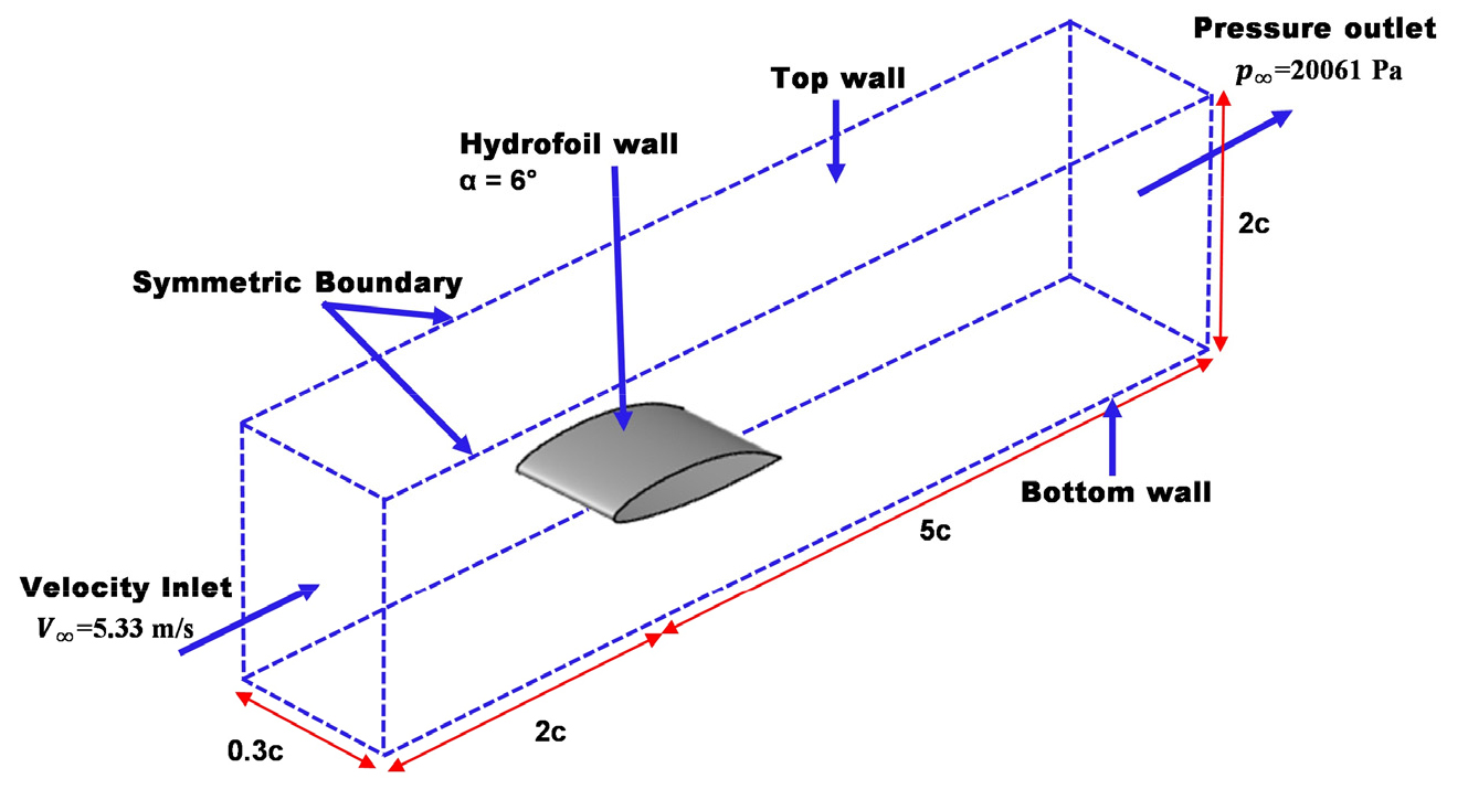
The computational domain with the boundary conditions around NACA66 hydrofoil which has a relative maximum thickness of 12% and a relative maximum camber of 2% is represented in Fig. 1. The angle of attack (𝛼=6°) and the chord length of the hydrofoil is $c$ =0.15[m]. The inlet and outlet is located at the distance of 2 $c$ and 5 $c$ from the leading edge, respectively. The span-wise length is selected as 0.3 $c$ since the span-wise length should be more than twice the hydrofoil thickness to resolve the stream-wise vortices. The height is selected as 2 $c$ which is sufficient to avoid the interaction of the wall [18].

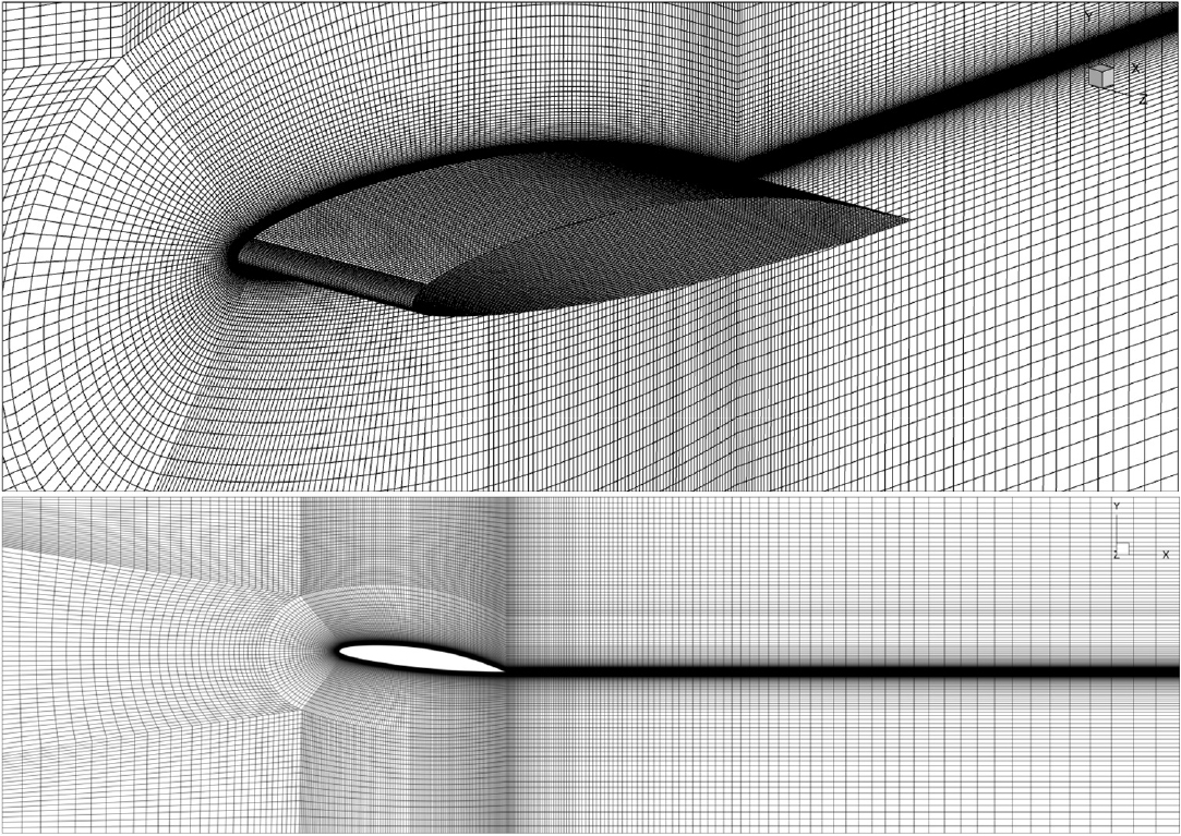
The O-H type mesh generation around NACA66 hydrofoil is shown in Fig. 2. The total number of grids is 3.4 million cells where the wall $Y^{+}$ value is less than 1 ( $Y^{+}$ ≈0.7) and the distance from the wall to the first grid is 3.6×10^-6 [m]. The number of grids in streamwise and spanwise on the surface of hydrofoil is 300×60 cells.

https://cdn.apub.kr/journalsite/sites/kscfe/2024-029-03/N0500290311/images/jkscfe_2024_293_145_F1.jpg

Fig. 1.

Representation of the geometry and boundary conditions

https://cdn.apub.kr/journalsite/sites/kscfe/2024-029-03/N0500290311/images/jkscfe_2024_293_145_F2.jpg

Fig. 2.

O-H type mesh around NACA66 hydrofoil

The zones of roughness distribution on the suction side of the hydrofoil are illustrated in Fig. 3. The zone 1 is from $x / c$ =0~30%, the zone 2 is from $x / c$ =30~60%, and the zone 3 is from $x / c$ 60~100%. The roughness effects are examined with the various zone configurations which are the no roughness (case 1), the patch roughness (case 2), and three different roughness (case 3). The physical roughness heights ( $K_{S}$ ) applied in each zone are displayed in Table 1. The meaning of $K_{S}$ =0.8 [mm] and $K_{S}$ =1 [mm] represents the fully roughness condition which satisfies $K_{S}^{+}$ ≻90. The $K_{S}$ =0.2 [mm] is the transitional roughness condition (2.25≺ $K_{S}^{+}$ ≤902.25) and the $K_{S}$ =0[mm] is the fully smooth condition ( $K_{S}^{+}$ ≤2.25). The value of $K_{S}^{+}$ is calculated by eq. (18) with the physical roughness height( $K_{S}$ ) in Table 1 and the friction velocity( $u^{*}$ =0.18 [m/s]) calculated using Custom Field Function in the ANSYS for NACA66 hydrofoil.

https://cdn.apub.kr/journalsite/sites/kscfe/2024-029-03/N0500290311/images/jkscfe_2024_293_145_F3.jpg

Fig. 3.

The zone classification on the suction side of hydrofoil

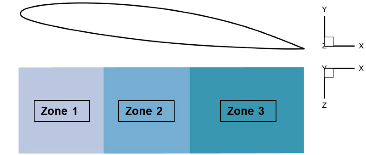
Table 1.

The various physical roughness distributions in three zones

	Physical Roughness height( $K_{S}$ ) [mm]
	Zone 1 (0-30%)	Zone 2 (30-60%)	Zone 3 (60-100%)
Case 1 (No Roughness)	0	0	0
Case 2 (Patch Roughness)	0	1 (full roughness)	0
Case 3 (3 Different Roughness)	0 (smooth roughness)	0.2 (transitional roughness)	0.8 (full roughness)

The inlet velocity $V_{\infty}$ is [m/s], the outlet pressure $p_{\infty}$ is 20061 [Pa], the reference cavitation number $σ_{\infty}$ is 1.249 calculated by $(σ_{\infty} = (p_{\infty} - p_{V}) / (0.5 ρ_{L} V_{\infty}^{2}))$ where $p_{V}$ is the saturated vapor pressure at $T$ =293.15 [K].

The numerical calculations for unsteady unstable cavitation flow begin with the converged solution for unsteady unstable non-cavitation flow. The time step size $∆ t$ =0.00005s is selected. The computer equipped with the Intel Core i9-13900K CPU which contains 24 cores and with 128 [GB] of RAM is used.

3. Results and Discussion

In order to investigate the roughness effects on unsteady unstable( $σ_{\infty}$ =1.249) partial cavitation flow around NACA66 hydrofoil, the Schnerr-Sauer cavitation model with LES model is used. The numerical model and computational domain used in this paper are already validated in the study of unsteady stable( $σ_{\infty}$ =1.34) cavitation flow compared with experimental results [14].

The suction side surface of the hydrofoil is divided into three zones (see Fig. 3). Zone 1 accelerates the flow where the sheet cavitation is usually developed on the surface. Zone 2 is a transitional zone where the attached sheet cavitation collapses due to the re-entry jet and the pressure change of the flow, forming cloud cavitation. Zone 3 is the aft region of the hydrofoil where the cloud cavitations are collapsed. No Roughness for all zones is used as reference case (case 1). Patch Roughness is given to study the roughness effect where sheet cavitation transforms into cloud cavitation (case 2). The violent collapse of cavitation bubbles in cloud cavitation generates high-impact loads on the surface of the material [19]. Cloud cavitation tends to produce greater surface roughness than sheet cavitation. To simulate this effect, three different roughness is applied (case 3).

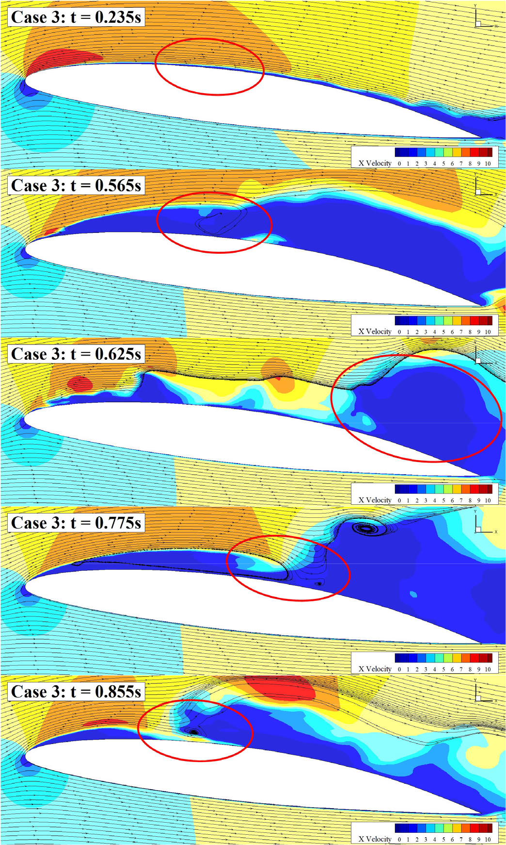
In all three cases, the converged solutions for the non-cavitating flow are first obtained by the time t = 0.5s where a fully developed turbulence flow is achieved. The converged solutions are then used as the initial conditions in the calculation of cavitation flow after the time t=0.5s. The streamline and velocity contours for water around NACA66 hydrofoil for case 3 are represented in Fig. 4. At the time t=0.235s, which is the non-cavitation flow, the stagnation zone of water is formed near the wall due to the no-slip condition. After the time t=0.5s, where the cavitation model is turned on, the cavitation cycle starts near the leading edge. The cavity flows downstream with a speed of $V$ =3.19 [m/s] at the initial stage of the cavity. The cavity acts as a vapor block and a stagnation zone of water. Fig. 4 depicts the collapse of the attached sheet cavitation caused by the re-entry jet and the pressure change in the flow.

https://cdn.apub.kr/journalsite/sites/kscfe/2024-029-03/N0500290311/images/jkscfe_2024_293_145_F4.jpg

Fig. 4.

The streamline and velocity contours for water around NACA66 hydrofoil

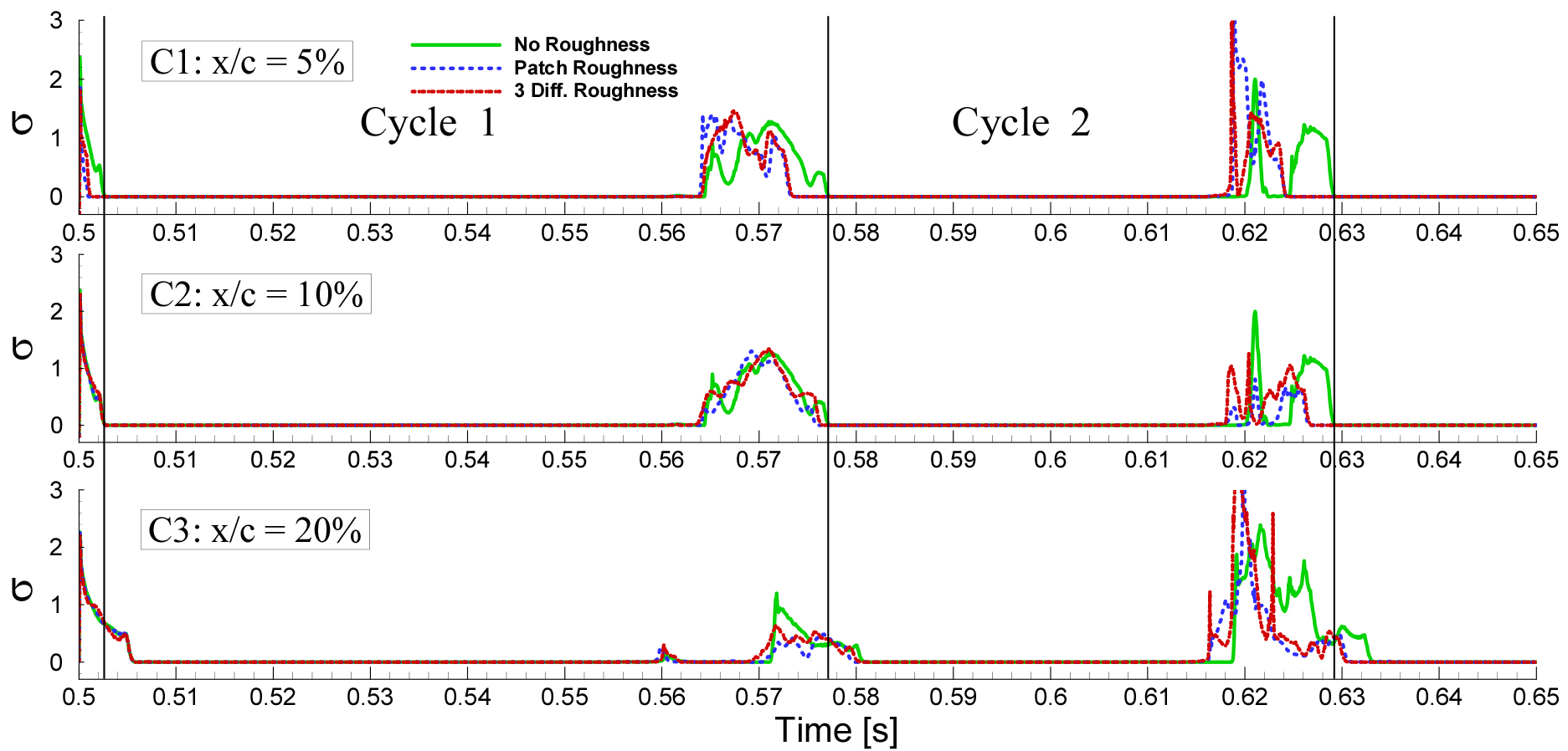
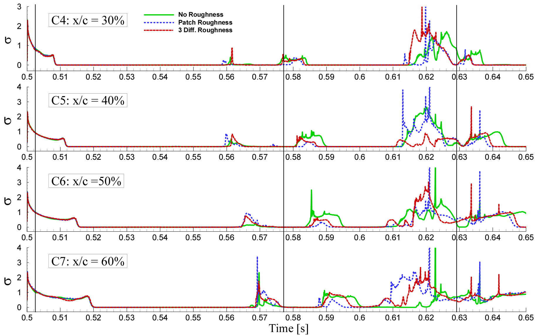
The distribution of local cavitation numbers ( $(σ = (p - p_{V}) / (0.5 ρ_{L} V_{\infty}^{2}))$ ) for each zone is depicted in Fig. 5, 6, and 7. The cavitation number is calculated over time at each location on the suction side of NACA66 hydrofoil, identical to the points illustrated in Leroux's experimental study [2]. The pressure is obtained just above the surface vertically. The points C1, C2, and C3 in Fig. 5 represent the locations of $x / c$ =5%, 10%, and 20%, respectively. The vertical line at the time t=0.503s, 0.577s, and 0.629s indicate the starting time of cavitation of case 1 (no roughness) at $x / c$ =5%. These lines are applied to all figures as a guideline. The cycle is defined as the period between the disappearance of the former cavitation and the development of new cavitation. This cycle is based on case 1 at $x / c$ =5%. The local cavitation number 𝜎=0 indicates the occurrence of cavitation, while the spike (𝜎≻0) indicates the collapse and condensation of the cavity in Fig. 5, 6, and 7. The starting times of cavitation for case 2 and 3 at $x / c$ =5% are the same (i.e. t=0.501s, 0.573s, and 0.624s) which are earlier than in case 1 during the cycle 1, 2, and 3. In Fig. 5, 6, and 7, specifically at the time t=0.52s, 𝜎=0 for case 2 (patch roughness) indicates that the cavity covers $x / c$ =5% to 60%of suction side surface, while 𝜎≻0 implies no cavity between $x / c$ =70% and 90% (see Fig. 8).

https://cdn.apub.kr/journalsite/sites/kscfe/2024-029-03/N0500290311/images/jkscfe_2024_293_145_F5.jpg

Fig. 5.

The change of local cavitation number over time in each point of zone 1

https://cdn.apub.kr/journalsite/sites/kscfe/2024-029-03/N0500290311/images/jkscfe_2024_293_145_F6.jpg

Fig. 6.

The change of local cavitation number over time in each point of zone 2

https://cdn.apub.kr/journalsite/sites/kscfe/2024-029-03/N0500290311/images/jkscfe_2024_293_145_F7.jpg

Fig. 7.

The change of local cavitation number over time in each point of zone 3

https://cdn.apub.kr/journalsite/sites/kscfe/2024-029-03/N0500290311/images/jkscfe_2024_293_145_F8.jpg

Fig. 8.

The 2D contours of cavity volume along the middle line of the span for case 2

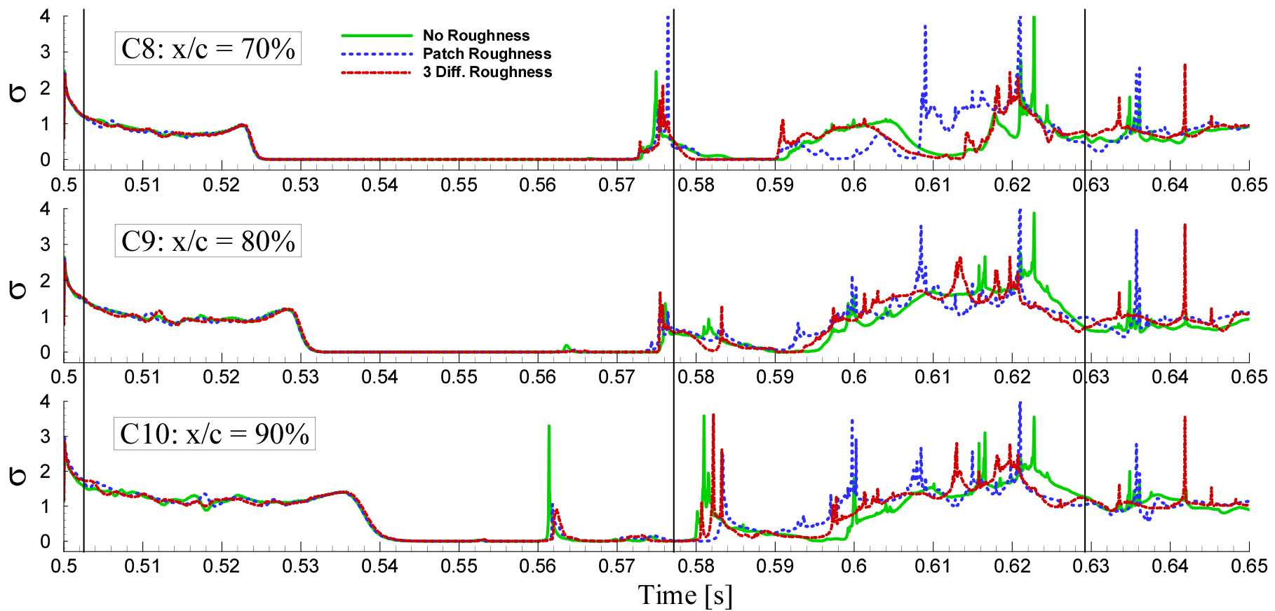
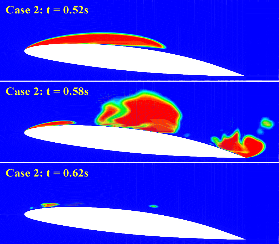
At the time t=0.62s, all locations from C1 to C10 for case 2 represent the spike (𝜎≻0) which means no cavity on the suction side except $x / c$ =10% where 𝜎=0 indicates (see Fig. 8). At another specific time t=0.58s, the location of $x / c$ =30%, 70%, and 80% for case 2 indicates 𝜎≻0. This phenomenon (𝜎≻0) coincides with the cavity behavior in Fig. 8 where the cavity does not exist in these locations. The distributions of cavity volume for case 2 at three specific times are shown in Fig. 8, demonstrating the phenomenon of unsteady partial cavitation.

The changes of cavity volume (vapor volume fraction) during 12 cycles is shown in Fig. 9. The cavity volume for the three cases remains constant during cycle 1 as this is the initial stage where the sheet cavitation travels from the leading edge to the trailing edge with an initial speed of $V$ =3.19 [m/s]. In cycle 1 and 2, the cavity volume reaches its maximum peak of 6.3 [10^-5m³]. After cycle 3, the maximum value of the cavity volume fluctuates below 3.6 [10^-5m³]. The sheet cavitation starts to collapse due to the pressure change in the flow as soon as it reaches the trailing edge. The sheet cavitation transforms into cloud cavitation and the cavitation flow becomes more complex. These changes show the variation in cavity volume from cycle 2 for three cases in Fig. 9. Also, the intervals of the cycles are not equal. After cycle 3, the significant changes in the cavity volume combined with roughness effects are observed.

https://cdn.apub.kr/journalsite/sites/kscfe/2024-029-03/N0500290311/images/jkscfe_2024_293_145_F9.jpg

Fig. 9.

The changes of vapor volume fraction during 12 cycles

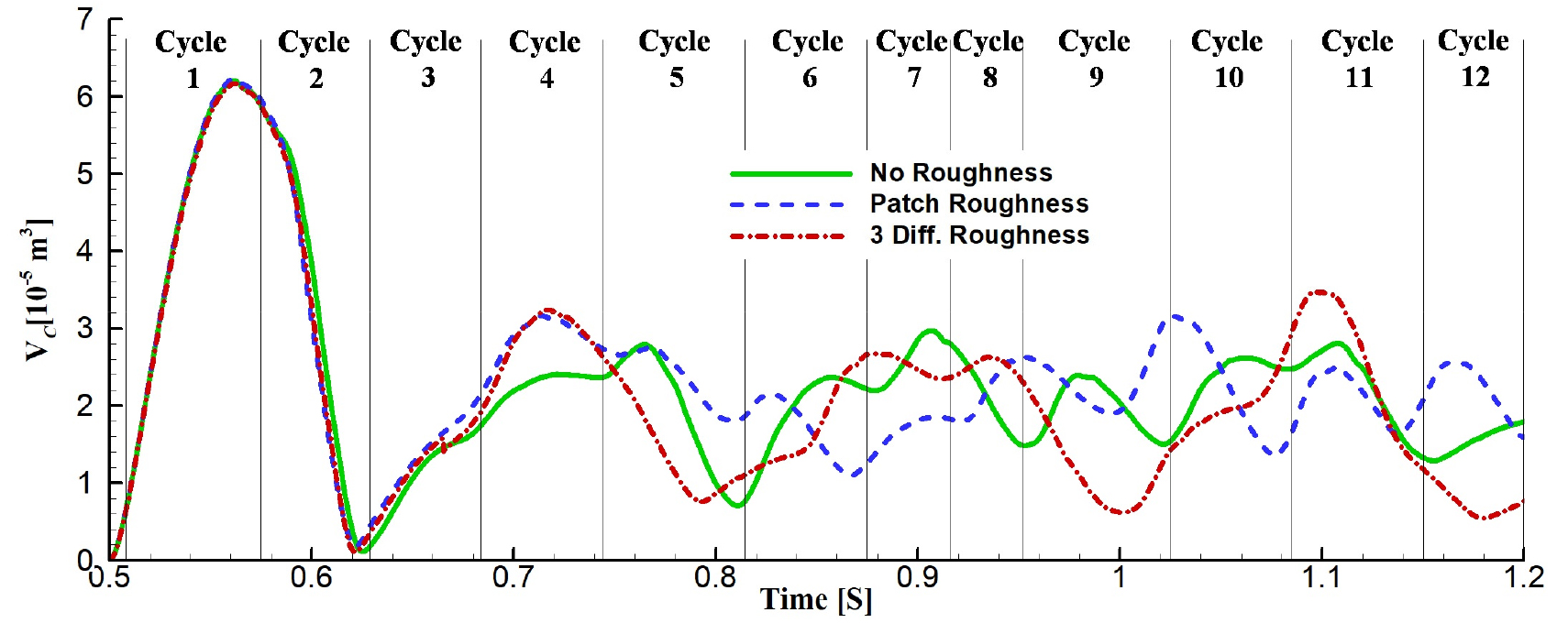
The cavity volume and corresponding cavity shedding times for the first 10 cycles are shown in Table 2. It is evident that the cavity volume is not proportional to the cavity shedding time and the shedding time is also non-uniform due to the nature of the unsteady partial cavity. The shedding frequency is defined as the number of cycles per second. The calculated values for cases 1, 2, and 3 are 15.6 [Hz], 15.7 [Hz], and 17.7 [Hz], respectively. Here, the shedding frequency increases as the distribution area of roughness increases (see Table 1). Such different frequencies are a result of roughness effects. Increased roughness surface causes higher turbulent velocity, which in turn destabilizes sheet cavitation, leading to faster cavitation collapse or shedding. The increased turbulence also enhances the effectiveness of the re-entrant jet, contributing to the breakdown of the sheet cavitation. As a result, increased roughness surface leads to higher shedding frequency.

Table 2.

Cavity volume $V_{c}$ and cavity shedding time $∆ t$ [s] during 10 cycles for each case

Cycle No.	No Roughness		Patch Roughness		3 Different roughness
Cycle No.	$V_{c} [m^{3}]$	$∆ t$ [s]	$V_{c} [m^{3}]$	$∆ t$ [s]	$V_{c} [m^{3}]$	$∆ t$ [s]
1	0.06220	0.074	0.05822	0.072	0.05803	0.072
2	0.02880	0.052	0.03296	0.051	0.03635	0.051
3	0.01052	0.046	0.01227	0.052	0.01121	0.056
4	0.03861	0.071	0.03561	0.064	0.02655	0.060
5	0.01953	0.070	0.03287	0.067	0.02465	0.051
6	0.02151	0.061	0.02041	0.057	0.01323	0.052
7	0.03812	0.076	0.01891	0.059	0.03207	0.066
8	0.01641	0.071	0.03163	0.069	0.02623	0.063
9	0.02424	0.061	0.03932	0.082	0.01586	0.036
10	0.03197	0.059	0.02590	0.064	0.02398	0.058

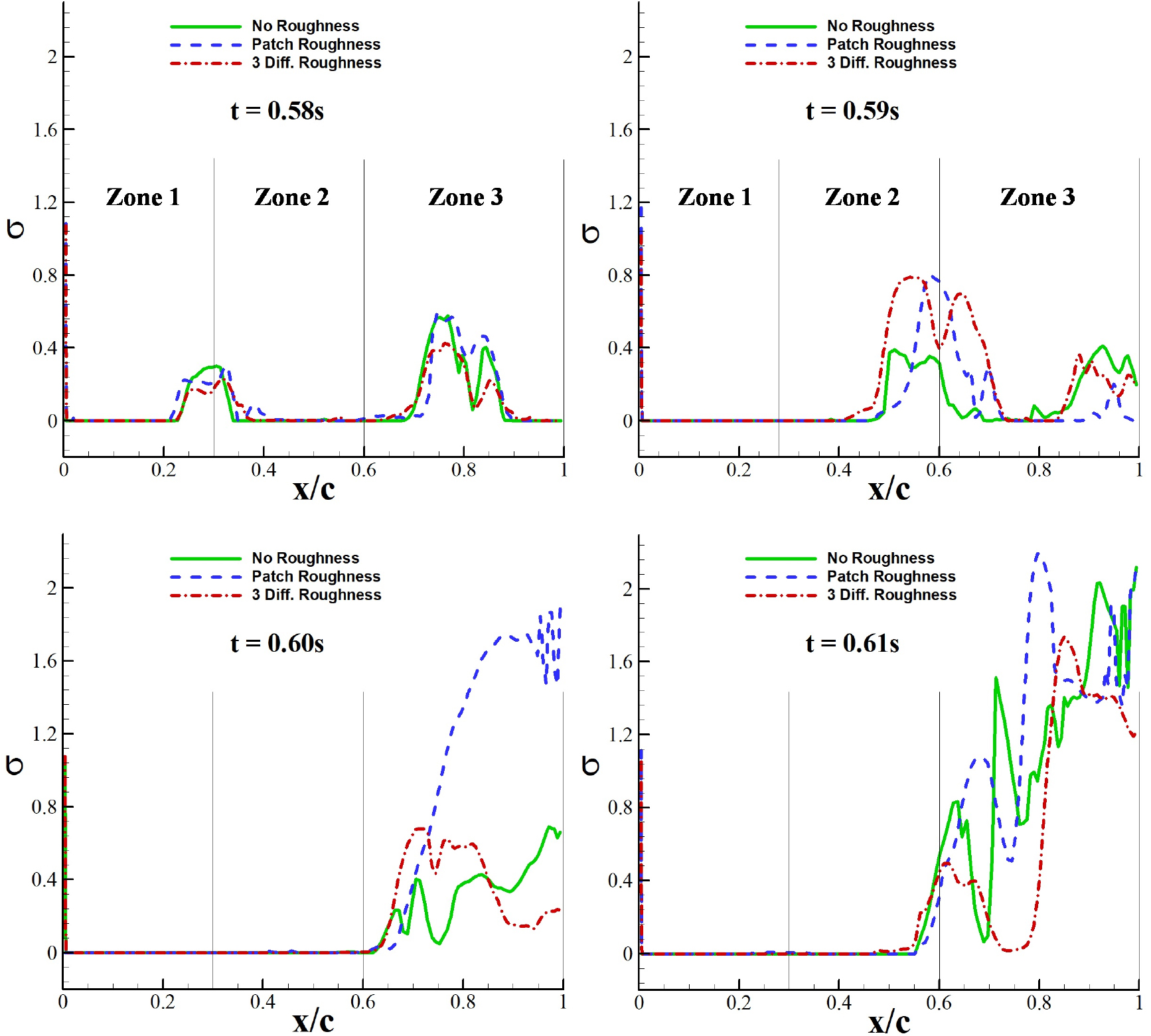
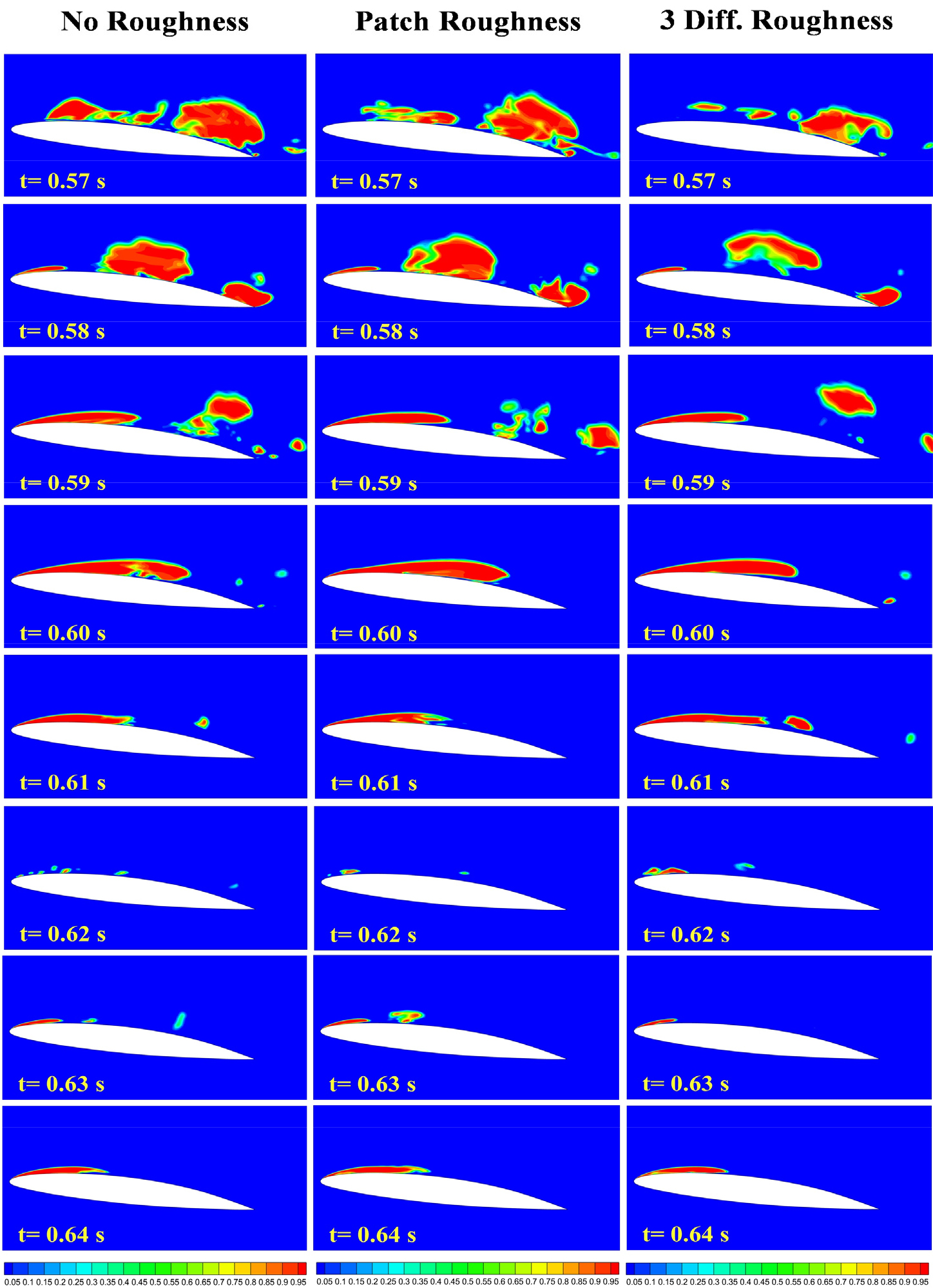
Fig. 10 shows the distributions of local cavitation number along the suction side of the hydrofoil at specific times. At the time t=0.58s, the spike (𝜎≻0) roughly between $x / c$ =20% and 40% and between 70% and 90% indicates no cavity. This phenomenon corresponds to the contours at the time t=0.58s in Fig. 11 and 12. The sheet cavitation covers approximately 50% of the surface at t=0.59s and roughly 65% of the surface at the time t=0.60s in Fig. 10, 11, and 12. At t=0.61s, the cavity fragment is located roughly at $x / c$ =70% for case 1, at $x / c$ =73%~78% for case 3, and no cavity fragment for case 2. All cases in zone 1 have no roughness (see Table 1). The local cavitation numbers in this zone behave similarly at each time. Also, case 1 and 2 in zone 3 have no roughness but the behaviors of 𝜎 are quite different. In cycle 2, the pressure changes have a greater influence on the cavitation behavior than the roughness effect.

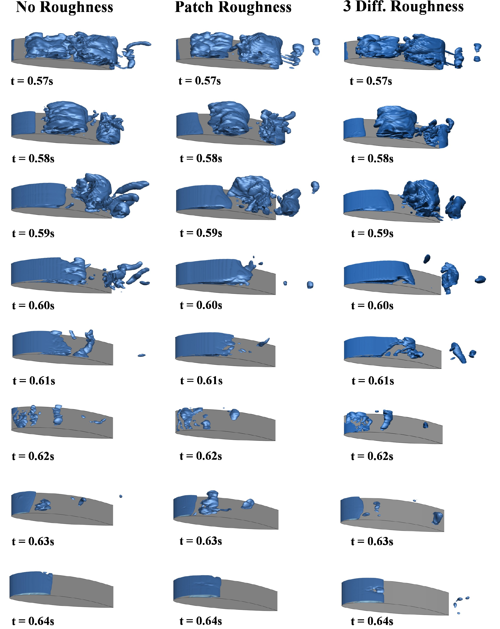
The 3D contours in Fig. 11 illustrate the evolution in cavity volume on the suction side of the hydrofoil between t=0.52 and t=0.64s and the 2D contours are shown in Fig. 12. The minimal differences in the cavity for the three cases are observed in 2D and 3D contours. The mechanism of unsteady partial cavitation behavior in the early stage can roughly be understood by matching these contours with the graphs in Fig. 5, 6, and 7.

https://cdn.apub.kr/journalsite/sites/kscfe/2024-029-03/N0500290311/images/jkscfe_2024_293_145_F10.jpg

Fig. 10.

The distributions of local cavitation number along the suction side of hydrofoil

https://cdn.apub.kr/journalsite/sites/kscfe/2024-029-03/N0500290311/images/jkscfe_2024_293_145_F11.jpg

Fig. 11.

The 3D contours of vapor volume fraction for three cases on the suction side of hydrofoil

https://cdn.apub.kr/journalsite/sites/kscfe/2024-029-03/N0500290311/images/jkscfe_2024_293_145_F12.jpg

Fig. 12.

The 2D contours of vapor volume fraction for three cases along the middle line of the span

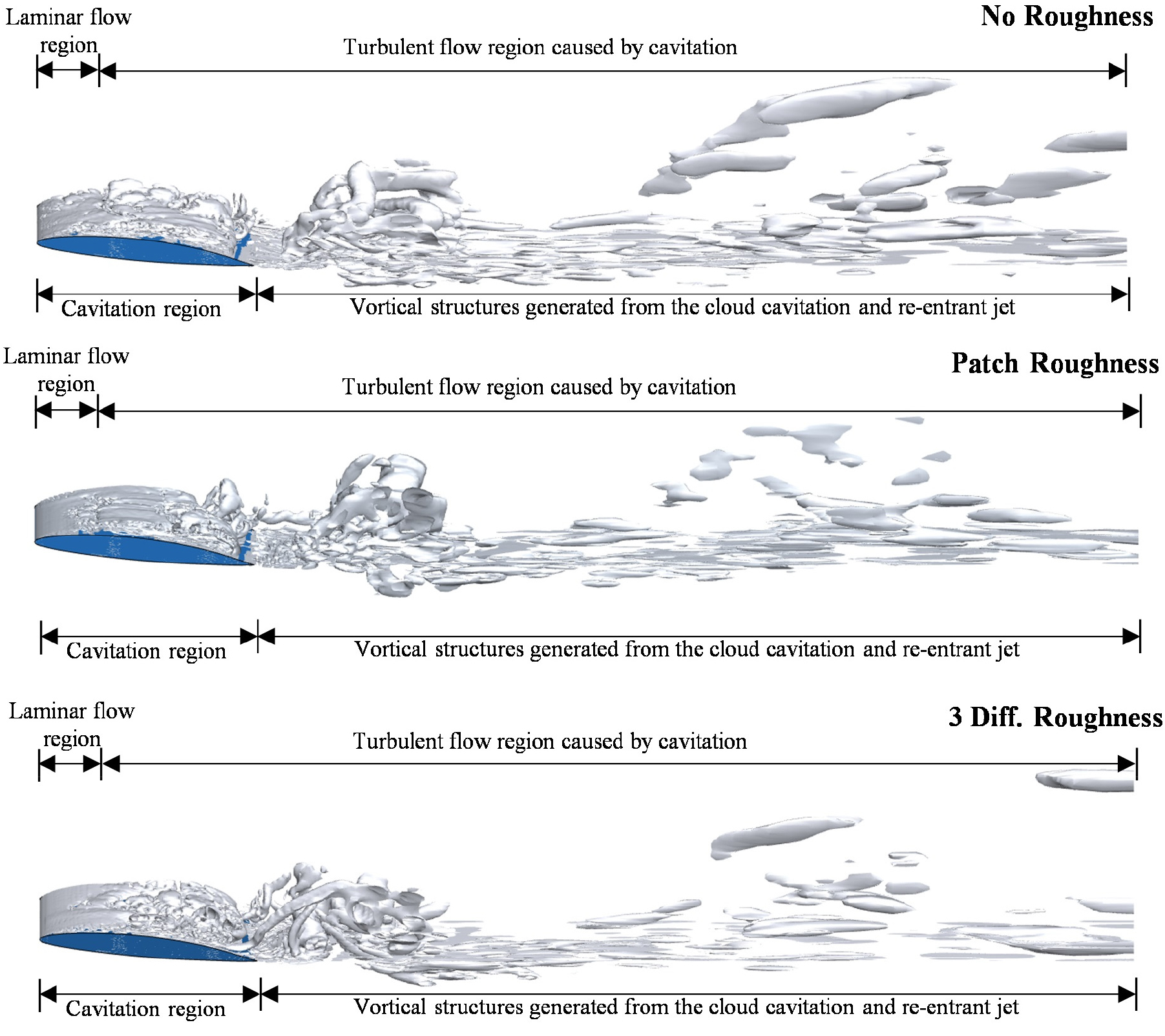
The roughness of the surface can affect the development of the boundary layer and flow separation, which may impact the creation and strength of vortices. The Q-criterion is used to identify vortices by measuring regions where rotation dominates overstrain. In Fig. 13, the cavitation region captures the vortical structures in both the vapor bubbles and the surrounding liquid. The Q-criterion in this area highlights vortices that coexist in both the liquid and vapor phases produced by cavitation. The vortical structures are not present in the region of laminar flow during the development of sheet cavitation. The re-entry jet formation and the rotational movement of cloud cavitation at the trailing edge result in increased rotational motion. The Q-criterion contours show no significant differences among the three cases with roughness effects due to changes in the cavitation cycle at the time t = 0.73s and due to the highly turbulent nature of the flow field.

https://cdn.apub.kr/journalsite/sites/kscfe/2024-029-03/N0500290311/images/jkscfe_2024_293_145_F13.jpg

Fig. 13.

The turbulent vortical flow structures induced by cavity shedding for all three cases (iso-surfaces $Q$ , 𝜎=1.249, and 𝛼=6°) at the time t = 0.73s

4. Conclusion

In this paper, the correlations between the roughness effects and cavity behavior with different roughness conditions are numerically investigated using the Schnerr-Sauer cavitation model with the LES turbulence model. The numerical results are analyzed through the local cavitation number(𝜎), vapor volume fraction, and 2D & 3D contours. The distribution of local cavitation numbers for the three cases at each zone illustrates the cavity behavior during cycles 1 and 2. The cavity pulsates abnormally and the periodic changes in the attached cavity length affect the cavitation occurrence significantly. The increased surface roughness leads to higher turbulent velocity. The turbulence destabilizes the sheet cavitation, leading to more rapid cavitation collapse or shedding. The increased turbulence enhances the effectiveness of the re-entrant jet which contributes to the breakdown of the sheet cavitation. When the local cavitation number 𝜎=0, the cavity appears. At the same time, when the local cavitation number 𝜎≻0 , no cavitation occurs and condensation occurs on the surface of the hydrofoil. These phenomena are observed the same in the 2D & 3D contours.

As a result, the higher shedding frequency occurs with the increased roughness area. The correlations between the distributions of local cavitation numbers along the surface and the 2D & 3D contours explain the cavitation phenomena physically. The Q-criterion contours show no significant differences among the three cases with roughness effects due to the highly turbulent nature of the flow field.

Acknowledgements

This work was supported by a Research Grant of Andong National University.

References

2009, Wright, T. and Gerhart, P.M., Fluid Machinery-Application, Selection, and Design, CRC Press.

2004, Leroux, J.B., Astolfi, J.A. and Billard, J.Y., "An Experimental Study of Unsteady Partial Cavitation," J. Fluids Eng., Vol.126, pp.94-101.

10.1115/1.1627835

1965, Numachi, F., Oba, R. and Chida, I., "Effect of Surface Roughness on Cavitatiion Performance of Hydrofoils -Report 1," J. Basic Eng., Vol.87, No.2, pp.495-503.

10.1115/1.3650583

2003, Stutz, B., "Influence of Roughness on the Two-Phase Flow Structure of Sheet Cavitation," J. Fluids Eng., Vol.125, pp.652-659.

10.1115/1.1596240

2009, Williams, M., Kawakami, E., Arndt, R. and Amromin, E., "Effects of Surface Characteristics on Hydrofoil Cavitation," In: Proceedings of the 7^th International Symposium on Cavitation CAV2009, Michigan, USA.

2016, Churkin, S., Pervunin, K.S. and Kravtsova, A. et al., "Cavitation on NACA0015 hydrofoils with different wall roughness: high-speed visualization of the surface texture effects," J. Vis., Vol.19, pp.587-590.

10.1007/s12650-016-0355-9

2018, Hao, J., Zhang, M. and Huang, X., "The influence of surface roughness on cloud cavitation flow around hydrofoils," Acta Mech. Sin., Vol.34, pp.10-21.

10.1007/s10409-017-0689-0

2011, Echouchene, F., Belmabrouk, H., Le Penven, L. and Buffat, M., "Numerical simulation of wall roughness effects in cavitating flow," Intl. J. of Heat and Fluid Flow, Vol.32, pp.1068-1075.

10.1016/j.ijheatfluidflow.2011.05.010

2020, Asnaghi, A. and Bensow, R.E., "Impact of Leading Edge Roughness in Cavitation Simulations around a Twisted Foil," Fluids, Vol.5, No.243, pp.1-18.

10.3390/fluids5040243

2021, Sun, Z.C., Mao, Y.F. and Fan, M.H., "Performance optimization and investigation of flow phenomena on tidal turbine blade airfoil considering cavitation and roughness," Appl. Ocean Res., Vol.106, pp.1-17.

10.1016/j.apor.2020.102463

1997, Kawanami, Y., Kato, H., Yamaguchi, H., Tanimura, M. and Tagaya, Y., "Mechanism and Control of Cloud Cavitation," J. Fluids Eng., Vol.119, pp.788-794.

10.1115/1.2819499

2003, Coutier, D.O., Reboud, J.L. and Delannoy, Y., "Numerical Simulation of the Unsteady Behaviour of Cavitating Flows," Int J. Numerical Methods in Fluids, Vol.42, pp.527-548.

10.1002/fld.530

2001, Schnerr, G.H. and Sauer, J., "Physical and Numerical Modeling of Unsteady Cavitation Dynamics. In: Proceedings of 4th International Conference on Multiphase Flow," New Orleans, USA.

2024, Karthik, V. and Lee, J.C., "Numerical Study of Unsteady Cavitation Characteristics Around NACA66 Hydrofoil Using LES Model," J. Computational Fluids Eng.,Vol.29, pp.90-99.

10.6112/kscfe.2024.29.1.090

1999, Nicoud, F. and Ducros, F., "Subgrid-Scale Stress Modelling Based on the Square of the Velocity Gradient Tensor," Flow, Turbul. and Combustion, Vol.62, pp.183-200.

10.1023/A:1009995426001

2024, Ansys, Ansays Fluent Theory Guide Machinery-Application, Selection, and Design, Ansys.

1998, Patel, V. C., "Perspective: Flow at High Reynolds Number and Over Rough Surfaces-Achilles Heel of CFD," J. Fluids Eng., Vol.120, pp.434-444.

10.1115/1.2820682

2002, Sagaut, P., Large Eddy Simulation for Incompressible Flows, Third edition, Springer, New york, USA.

2014, Bark, G. and Bensow, R.E., Hydrodynamic Processes Controlling Cavitation Erosion. In: Kim, KH., Chahine, G., Franc, JP., Karimi, A. (eds) Advanced Experimental and Numerical Techniques for Cavitation Erosion Prediction, Fluid Mechanics and Its Applications, Vol.106, pp.185-220, Springer, Dordrecht, Netherlands.

10.1007/978-94-017-8539-6_8

Journal of Computational Fluids Engineering ISSN:1598-6071(Print) 3022-6252(Online) 한국전산유체공학회지

Preview

ROUGHNESS EFFECTS ON UNSTEADY PARTIAL CAVITATION FLOW AROUND NACA66 HYDROFOIL USING THE LES MODEL

ABSTRACT

MAIN

(1)

(2)

(3)

(4)

(5)

(6)

(7)

(8)

(9)

(10)

(11)

(12)

(13)

(14)

(15)

(16)

(17)

(18)

(19)

(20)

Fig. 1.

Representation of the geometry and boundary conditions

Fig. 2.

O-H type mesh around NACA66 hydrofoil

Fig. 3.

The zone classification on the suction side of hydrofoil

Table 1.

The various physical roughness distributions in three zones

Fig. 4.

The streamline and velocity contours for water around NACA66 hydrofoil

Fig. 5.

The change of local cavitation number over time in each point of zone 1

Fig. 6.

The change of local cavitation number over time in each point of zone 2

Fig. 7.

The change of local cavitation number over time in each point of zone 3

Fig. 8.

The 2D contours of cavity volume along the middle line of the span for case 2

Fig. 9.

The changes of vapor volume fraction during 12 cycles

Table 2.

Cavity volume Vc and cavity shedding time ∆t [s] during 10 cycles for each case

Fig. 10.

The distributions of local cavitation number along the suction side of hydrofoil

Fig. 11.

The 3D contours of vapor volume fraction for three cases on the suction side of hydrofoil

Fig. 12.

The 2D contours of vapor volume fraction for three cases along the middle line of the span

Fig. 13.

The turbulent vortical flow structures induced by cavity shedding for all three cases (iso-surfaces Q, 𝜎=1.249, and 𝛼=6°) at the time t = 0.73s

Acknowledgements

References

Cavity volume $V_{c}$ and cavity shedding time $∆ t$ [s] during 10 cycles for each case

The turbulent vortical flow structures induced by cavity shedding for all three cases (iso-surfaces $Q$ , 𝜎=1.249, and 𝛼=6°) at the time t = 0.73s